The double exponential function has great versatility in generating a remarkable range of waveshapes. In general the form of the equation is shown here where E, a, and b are arbitrary complex constants.
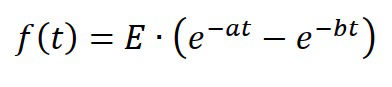
The double exponential function has great versatility in generating a remarkable range of waveshapes. In general the form of the equation is shown here where E, a, and b are arbitrary complex constants.
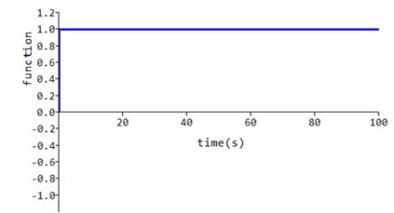
Heavyside’s unit step function
In this case the real part of a is zero, the real part of b is infinity, the real part of e is one, and the imaginary parts of a, b and c are all zero.
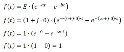
In numerical work, due to floating point arithmetic it is not possible to set the real part of b to infinity, however with:
a = (0.0 + j 0.0)
b = (1000 + j 0.0) (i.e. relatively large real part), and
e = (1.0 + j 0.0)
the curve shown is obtained which is clearly the unit step function.
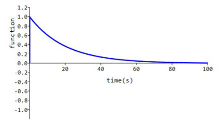
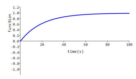
Simple decaying exponential wave
In this case the real part of a is non-zero, the real part of b is infinity, the real part of e is one, and the imaginary parts of a, b, and c are all zero.
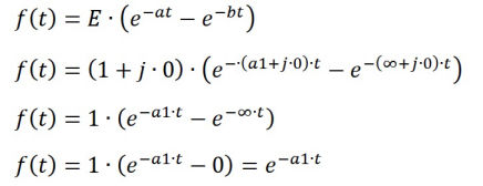
With :
a = (0.05 + j 0.0),
b = (1000 + j 0.0) (i.e. relatively large real part), and
e = (1.0 + j 0.0)
the curve shown is obtained which is a decaying exponential function.
This curve could represent the decay of current in a series resistor-capacitor circuit with a resistance of 1 ohm and the capacitor selected to give a circuit time constant of 20 s (i.e. 1/0.05 = 20) when the circuit is energised by a dc voltage source of 1 V.
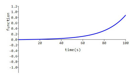
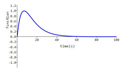
Convex rising front wave
This waveform can be obtained by setting the real and imaginary parts of a and the imaginary part of b to zero, while adjusting the real part of b to give a front of the desired length.
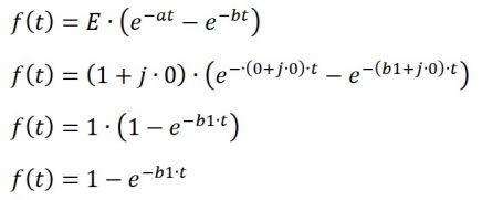
With:
a = (0.0 + j 0.0),
b = (0.05 + j 0.0) (i.e. relatively small real part), and
e = (1.0 + j 0.0)
the curve shown is obtained.
This curve represents the build-up of voltage across the capacitor in a series resistor-capacitor circuit with a resistance of 1 ohm and the capacitor selected to give a circuit time constant of 20 s (i.e. 1/0.05 = 20) when the circuit is energised by a dc voltage source of 1 V.
Concave rising front wave
This waveform can be obtained by setting the real part of a to -k and real part of b to +k, and the imaginary parts of a, b, and e to zero, with the real part of e equal to a non-zero value, which results in the double exponential function generating the hyperbolic sine function sinh(kt).
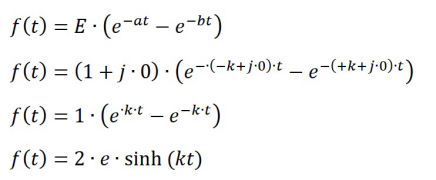
With:
a = (-0.05 + j 0.0),
b = (0.05 + j 0.0), and
e = (0.006 + j 0.0)
the curve shown is obtained.
Linear front (ramp) wave
A linear front or ramp wave i.e. constant rising slope can be obtained by setting a = (0.00, j0.00), and letting the real part of b tend to zero and e tend to infinity in such a way that the product bE remains finite.
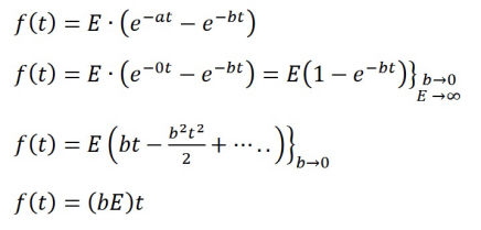
With
a = (0.0 + j 0.0),
b = (0.0001 + j 0.0), and
e = (10000 + j 0.0)
the curve shown is obtained.
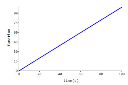
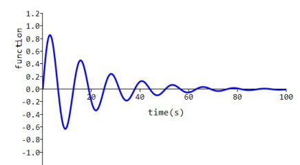
Damped sinusoidal wave
A damped sinusoidal wave is obtained by setting a = (α + jω), b = (α - jω) and
E = Eo/(2j) = -j∙0.5∙Eo
With:
a = (0.05 - j 0.5),
b = (0.05 + j 0.5), and
e = (0.0 – j 0.5)
the damped sinusoidal curve shown is obtained.
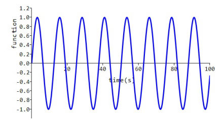
Sustained sinusoidal wave
A sustained sinusoidal wave is obtained by setting a = (α + jω), b = (α - jω) where α = 0 and E = Eo/(2j) = -j∙0.5∙Eo
With
a = (0.0 - j 0.5),
b = (0.0 + j 0.5), and
e = (0.0 – j 0.5)
the sustained sinusoidal curve shown is obtained.
In this case ω = 0.5, so ω/(2π) = 0.08 Hz, and there are approximately 8 cycles of this wave in 100 s.
Rounded front and exponential tail wave
Finally if a, b, and E are all finite and real, the double exponential formula provides the familiar lightning waveform with a rounded front and an exponential tail. The three parameters a, b, and E are sufficient to determine uniquely the crest, front, and tail of the wave.
As an example with
a = (0.1 + j 0.0),
b = (0.2 + j 0.0), and
E = (4.0 + j 0.0)
the waveshape is as shown.
While the pervious example shows the correct waveshape for a lightning wave, its duration is significantly longer than a lightning wave. The “standard” lightning waves can be obtained by appropriate scaling of the parameters a, b, and E.
Summary
The double exponential functioncan be used to synthesise a wide range of waveforms including:
Heavyside’s unit step function
A decaying exponential wave
A convex rising front wave
A concave rising front wave
A linear front (ramp) wave
A damped sinusoidal wave
A sustained sinusoidal wave
A rounded front and exponential tail wave (lightning wave)
The double exponential function is extremely versatile from a modelling perspective as all of these different waveforms are obtained by simply adjusting three complex numbers!
Last updated: 22/01/2022
Disclaimer
The information presented in this technical note is for educational purposes only.
K S Power Consulting Ltd. disclaims any responsibility and liability resulting from the use and interpretation of this information.